Basic Concepts

In this section, we explain the basic elements of the autonomous-learning-library and the philosophy behind some of the basic design decision.

Agent-Based Design

One of the core philosophies in the autonomous-learning-library is that RL should be agent-based, not algorithm-based. To see what we mean by this, check out the OpenAI Baselines implementation of DQN. There’s a giant function called learn which accepts an environment and a bunch of hyperparameters, at the heart of which there is a control loop which calls many different functions. Which part of this function is the agent? Which part is the environment? Which part is something else? We call this implementation algorithm-based because the central abstraction is a function called learn which provides the complete specification of an algorithm. What should the proper abstraction for agent be, then? We have to look no further than the following famous diagram from the Sutton and Barto textbook:

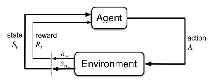
The definition of an Agent is simple. It accepts a state and reward, and returns an action. That’s it. Everything else is an implementation detail. Here’s the Agent interface in the autonomous-learning-library:

class Agent(ABC):
    @abstractmethod
    def act(self, state):
        pass

The act function is called when training the agent. When and how the Agent trains inside of this function is nobody’s business except the Agent itself. When the Agent is allowed to act is determined by some outer control loop, and is not of concern to the Agent. What might an implementation of act look like? Here’s the act function from our DQN implementation:

def act(self, state):
    self.replay_buffer.store(self._state, self._action, state)
    self._train()
    self._state = state
    self._action = self.policy.no_grad(state)
    return self._action

That’s it. _train() is a private helper methods. There is no reason for the control loop to know anything about these details. There is no tight coupling between the Agent and the control loop. This approach simplifies both our Agent implementation and the control loop itself.

Separating the control loop logic from the Agent logic allows greater flexibility in the way agents are used. In fact, Agent is entirely decoupled from the Environment interface. This means that our agents can be used outside of standard research environments, such as part of a REST API, a multi-agent system, etc. Any code that passes a State is compatible with our agents.

What is a State? The State abstraction is part of all.core and it represents all of the information available to the agent at a given timestep. It contains some default entries, including state['observation'], state['reward'], and state['done'], and state['mask']. A StateArray object can be constucted by calling State.array(list_of_states), and provides an abstraction for batch processing of states. Arbitrary entries can be added to a State, and use of the StateArray abstraction ensures that these entries are combined and sliced properly. The code does not need to be tightly coupled to the shape of the data, but rather can act on the abstraction.

Parallel Agents and Multiagents

We described above the base Agent interface. However, some algorithms do not fit this interface. For example, a ParallelAgent accepts a StateArray rather than a State. A Multiagent accepts a State object containing a special Agent key indicating to which of the multiagents the current state belongs, we we call a MultiagentState. Nevertheless, we stick to the spirit of having a single act() function as closely as possible. The resulting interfaces are as follows:

class ParallelAgent(ABC):
    @abstractmethod
    def act(self, state_array):
        pass

class Multiagent(ABC):
    @abstractmethod
    def act(self, multiagent_state):
        pass

Function Approximation

Almost everything a deep reinforcement learning agent does is predicated on function approximation.

For this reason, one of the central abstractions in the autonomous-learning-library is Approximation. By building agents that rely on the Approximation abstraction rather than directly interfacing with PyTorch Module and Optimizer objects, we can add to or modify the functionality of an Agent without altering its source code (this is known as the Open-Closed Principle). The default Approximation object allows us to achieve a high level of code reuse by encapsulating common functionality such as logging, model checkpointing, target networks, learning rate schedules and gradient clipping. The Approximation object in turn relies on a set of abstractions that allow users to alter its behavior. Let’s look at a simple usage of Approximation in solving a very easy supervised learning task:

import torch
from torch import nn, optim
from all.approximation import Approximation

# create a pytorch module
model = nn.Linear(16, 1)

# create an associated pytorch optimizer
optimizer = optim.Adam(model.parameters(), lr=1e-2)

# create the function approximator
f = Approximation(model, optimizer)

for _ in range(200):
    # Generate some arbitrary data.
    # We'll approximate a very simple function:
    # the sum of the input features.
    x = torch.randn((16, 16))
    y = x.sum(1, keepdim=True)

    # forward pass
    y_hat = f(x)

    # compute loss
    loss = nn.functional.mse_loss(y_hat, y)

    # backward pass
    f.reinforce(loss)

Easy! Now let’s look at the _train() function for our DQN agent:

def _train(self):
    if self._should_train():
        # sample transitions from buffer
        (states, actions, rewards, next_states, _) = self.replay_buffer.sample(self.minibatch_size)

        # forward pass
        values = self.q(states, actions)

        # compute targets
        targets = rewards + self.discount_factor * torch.max(self.q.target(next_states), dim=1)[0]

        # compute loss
        loss = self.loss(values, targets)

        # backward pass
        self.q.reinforce(loss)

Just as easy! The agent does not need to know anything about the network architecture, logging, regularization, etc. These are all handled through the appropriate configuration of Approximation. Instead, the Agent implementation is able to focus exclusively on its sole purpose: defining the RL algorithm itself. By encapsulating these details in Approximation, we are able to follow the single responsibility principle.

A few other quick things to note: f.no_grad(x) runs a forward pass with torch.no_grad(), speeding computation. f.eval(x) does the same, but also puts the model in eval mode first, (e.g., BatchNorm or Dropout layers), and then puts the model back into its previous mode before returning. f.target(x) calls the target network (an advanced concept used in algorithms such as DQN. For example, David Silver’s course notes) associated with the Approximation, also with torch.no_grad(). The autonomous-learning-library provides a few thin wrappers over Approximation for particular purposes, such as QNetwork, VNetwork, FeatureNetwork, and several Policy implementations.

ALL Environments

The importance of the Environment in reinforcement learning nearly goes without saying. In the autonomous-learning-library, the prepackaged environments are simply wrappers for Gymnasium (formerly OpenAI Gym), the defacto standard library for RL environments.

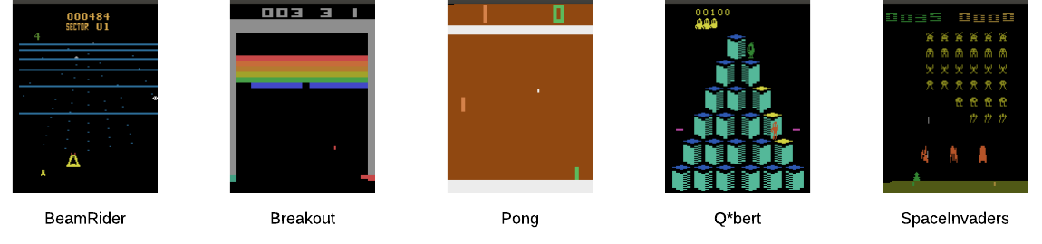
Some environments included in the Atari suite in Gym. This picture is just so you don’t get bored.

We add a few additional features:

1. gymnasium primarily uses numpy.array for representing states and actions. We automatically convert to and from torch.Tensor objects so that agent implemenetations need not consider the difference.

2. We add properties to the environment for state, reward, etc. This simplifies the control loop and is generally useful.

3. We apply common preprocessors, such as several standard Atari wrappers. However, where possible, we prefer to perform preprocessing using Body objects to maximize the flexibility of the agents.

Below, we show how several different types of environments can be created:

from all.environments import AtariEnvironment, GymEnvironment, MujocoEnvironment

# create an Atari environment on the gpu
env = AtariEnvironment('Breakout', device='cuda')

# create a classic control environment on the cpu
env = GymEnvironment('CartPole-v0')

# create a PyBullet environment on the cpu
env = MujocoEnvironment('HalfCheetah-v4')

Now we can write our first control loop:

# initialize the environment
env.reset()

# Loop for some arbitrary number of timesteps.
for timesteps in range(1000000):
    env.render()
    action = agent.act(env.state)
    env.step(action)

    if env.done:
        # terminal update
        agent.act(env.state)

        # reset the environment
        env.reset()

Of course, this control loop is not exactly feature-packed. Generally, it’s better to use the Experiment module described later.

ALL Presets

In the autonomous-learning-library, agents are compositional, which means that the behavior of a given Agent depends on the behavior of several other objects. Users can compose agents with specific behavior by passing appropriate objects into the constructor of the high-level algorithms contained in all.agents. The library provides a number of functions which compose these objects in specific ways such that they are appropriate for a given set of environment. We call such a function a preset, and several such presets are contained in the all.presets package. (This is an example of the more general factory method pattern).

For example, all.agents.dqn contains a high-level description of the DQN algorithm. However, how do we actually instansiate a particular network architecture, choose a learning rate, etc.? This is what presets are for. Before we dive into the details, let us show the simplest usage in practice:

from all.presets.atari import dqn
from all.environments import AtariEnvironment

# create an environment
env = AtariEnvironment('Breakout')

# configure and build the preset
preset = dqn.env(env).build()

# use the preset to create an agent
agent = preset.agent()

Instansiating the Agent is separated into two steps: First we configure and build the Preset, then we use the configured Preset to instansiate an Agent. Let’s dig into the Preset interface first:

class Preset(ABC):
    @abstractmethod
    def agent(self, logger=None, train_steps=float('inf')):
        pass

    @abstractmethod
    def test_agent(self):
        pass

    def save(self, filename):
        return torch.save(self, filename)

The agent() method instansiates a training Agent. The test_agent() method instansiates a test-mode Agent using the same network parameters as the training Agent. The save() then allows the Preset to be saved to a disk. Critically, all agents created by a given instance of a Preset share the underlying network parameters. The test agents, however, will instead copy the parameters, allowing test agents to be compared from multiple points in training. If a Preset is loaded from disk, then we can instansiate a test Agent using the pre-trained parameters.

ALL Experiments

Finally, we have all of the components necessary to introduce the run_experiment helper function. run_experiment is the built-in control loop for running reinforcement learning experiment. It instansiates its own Logger object for logging, which is then passed to each of the presets, and runs each agent on each environment passed to it for some number of timesteps (frames) or episodes). Here is a quick example:

from all.experiments import run_experiment
from all.presets import atari
from all.environments import AtariEnvironment

agents = [
    atari.dqn,
    atari.ddqn,
    atari.c51,
    atari.rainbow,
    atari.a2c,
    atari.ppo,
]

envs = [AtariEnvironment(env, device='cuda') for env in ['BeamRider', 'Breakout', 'Pong', 'Qbert', 'SpaceInvaders']]

run_experiment(agents, envs, 10e6)

The above block executes each run sequentially. This could take a very long time, even on a fast GPU! If you have access to a cluster running Slurm, you can replace run_experiment with SlurmExperiment to speed things up substantially (the magic of submitting jobs is handled behind the scenes).

By default, run_experiment will write the results to ./runs. You can view the results in tensorboard by running the following command:

tensorboard --logdir runs

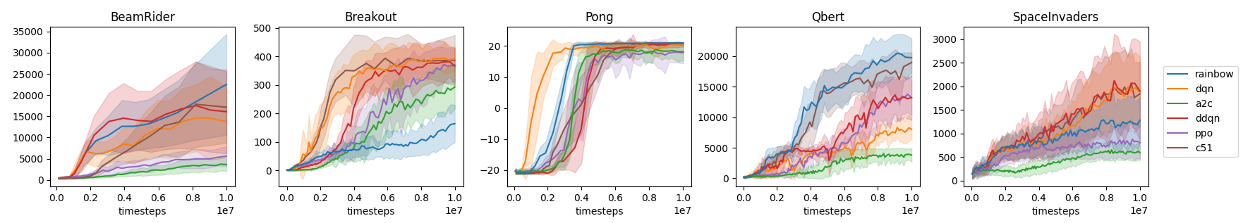
In addition to the tensorboard logs, every 100 episodes, the mean, standard deviation, min, and max of the previous 100 episode returns are written to runs/[agent]/[env]/returns100.csv. This is much faster to read and plot than Tensorboard’s proprietary format. The library contains an automatically plotting utility that generates appropriate plots for an entire runs directory as follows:

from all.experiments import plot_returns_100
plot_returns_100('./runs')

This will generate a plot that looks like the following (after tweaking the whitespace through the matplotlib UI):

An optional parameter is test_episodes, which is set to 100 by default. After running for the given number of frames, the agent will be evaluated for a number of episodes specified by test_episodes with training disabled. This is useful measuring the final performance of an agent.

You can also pass optional parameters to run_experiment to change its behavior. You can set render=True to watch the agent during training (generally not recommended: it slows the agent considerably!). You can set quiet=True to silence command line output. Lastly, you can set verbose=False to disable writing loss and debugging information to tensorboard. These files can become large, so this is recommended if you have limited storage!

Finally, run_experiment relies on an underlying Experiment API. If you don’t like the behavior of run_experiment, you can reuse the underlying Experiment objects to change it.